Deep Dive: Curve v2 Parameters

Curve v2 offers a host of parameters to optimize liquidity provision for various assets. What do these parameters do? A deep dive.

Overview

Curve v2 pools are designed to provide deep liquidity for a broad range of assets with varying degrees of volatility. Because different trading pairs can exhibit drastically different price dynamics, Curve v2 offers a variety of tunable parameters that can be used to optimize for different types of assets (see Curve Factory; Non-Pegged Assets). Here, I will go over each of these parameters so that users can have a basic understanding of how they work.

Do not be afraid, my child…

TL;DR

There are three classes of parameters to set when creating a Curve v2 pool:

1. Bonding Curve Parameters

   • A: controls liquidity concentration in the center of the bonding curve

   • Gamma: controls overall breadth of the curve; can fine-tune the extremes

2. Price Scaling Parameters

   • MA half time: controls the duration of the EMA internal “price oracle”

   • Allowed extra profit: excess profit (over the 50% baseline) required to allow price re-pegging

   • Adjustment step: minimum size of price scale adjustments

3. Fee Parameters

   • Fee mid: the minimum fee, charged when pool is fully balanced

   • Fee out: the maximum fee, charged when pool is fully imbalanced

   • Fee Gamma: controls how quickly fees increase (from fee mid to fee out) with greater imbalance

Three Components of Curve v2 Pools

Curve v2 pools consist of three core components: the bonding curve, the price scaling mechanism, and the fee mechanism. Each parameter adjusts a particular aspect of these three components. Here, I will briefly explain each component and how the relevant parameters alter their function.

1. The Bonding Curve

Overview

Like most AMMs, Curve v2 uses a bonding curve to price assets based on the pool’s supply of each asset. To concentrate liquidity near the center of the bonding curve, Curve v2 uses an invariant that is intermediate between the StableSwap (Curve v1) and constant-product (Uniswap, Balancer, etc.) invariants.

Comparison of AMM invariants: Curve v2 (orange), StableSwap (blue), and two constant product invariants (dashed). The line labelled “constant product” corresponds to the typical “xy=k” bonding curve. The line labelled “adj. constant product” is an adjusted constant product invariant that determines the asymptotic behavior at the “tails” of the v2 bonding curve. Modified from the whitepaper.

Notably, in contrast to other AMMs, the “center” (equilibrium point) of the Curve v2 bonding curve is dynamically shifted in accordance with price changes. This will be discussed in the “price scaling” section.

Parameters

The shape of the bonding Curve is governed by 2 parameters:

• A (amplification coefficient): As in the StableSwap invariant (Curve v1), the A parameter adjusts how flat the center portion of the bonding curve is. Therefore, it controls the concentration of liquidity near the expected exchange rate (i.e., the “price scale”; see below)

• Gamma: The gamma parameter adjusts the distance between the two constant product curves shown in the above figure (dashed lines). Increasing the gamma parameter “stretches” the “adjusted constant product” curve towards the lower-left corner of the graph, shifting the curve’s asymptotes closer to the axes and making the curve more broad overall

The effects of these parameters can be explored interactively here.

Effects of adjusting the A (left) and gamma (right) parameters. For the left plot, gamma = 0.000145. For the right plot, A = 400,000.

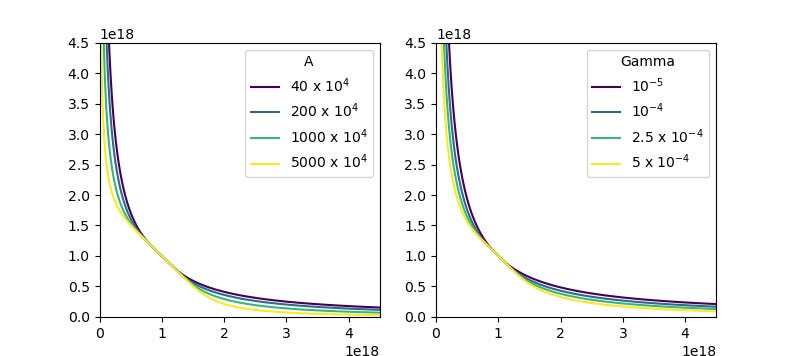
In general, the A parameter primarily adjusts the center portion of the curve, while the gamma parameter can be used to further fine-tune the overall shape. In particular, the gamma parameter can give more control over pricing as the pool becomes more imbalanced (i.e., towards the “tails” of the curve). However, these two parameters can have partially overlapping effects, especially when taken to the extreme. Generally, gamma should be kept very low (near zero).

2. Price Scaling

Overview

Curve v2 pools dynamically shift liquidity to maximize depth (i.e., minimize slippage) near current market prices. This is accomplished by taking a running EMA (exponential moving average) of the pool’s recent exchange rates (an “internal oracle”), and re-centering liquidity at the EMA only when it is financially reasonable for LPs to do so.

This process can be thought of as “re-pegging” the bonding curve so that the point of maximum liquidity concentration (i.e., the center of the curve) is matched to the EMA. The price where liquidity is maximally concentrated is referred to as the “price scale”, whereas the current EMA is referred to as the “price oracle.”

Price oracles and price scales for tricrypto2 pool at the time of writing. Note that “price scale” and “price oracle” can differ because price scales are only updated when certain conditions are met (see below).

Parameters

Three parameters govern price scaling in Curve v2.

First, the MA half time parameter adjusts the half-time of the EMA price oracle. This controls how temporally smoothed the price oracle is, with greater values increasing smoothing.

Second, the allowed extra profit and adjustment step parameters govern when re-pegging (i.e., updating “price scale” to equal “price oracle”) is allowed to occur. In particular, re-pegging only occurs if:

• Current profits are greater than half of feasible profits (i.e., profits ignoring losses due to re-pegging) plus the allowed extra profit parameter

• The price scale adjustment is larger than the adjustment step parameter (in units of log Euclidean distance between current and updated prices)

• Changing the price scale would retain at least half the pool’s profits

3. Fees

Overview

Curve v2 pools charge dynamic fees depending on pool balance/imbalance. Fees are minimal when the pool is in a balanced state, and increase with increasing imbalance.

Parameters

Dynamic fees are defined using three parameters:

• Fee Mid: The fee charged when the pool is completely balanced. This is the minimum fee.

• Fee Out: The fee charged when the pool is completely imbalanced. This is the maximum fee.

• Fee Gamma: Adjusts how quickly fees increase with greater imbalance. Lower values produce sharp fee increases with increased imbalance; higher values produce more gradual fee increases with increased imbalance.

An interactive example of these parameters is available here.

Schematic showing fees as a function of pool balance. As the pool goes from fully balanced (x-axis = 1) to fully imbalanced (x-axis = 0), fees increase from mid fee to out fee. The rate of increase is controlled by the fee gamma parameter.

Conclusions

Curve v2 provides a broad range of adjustable parameters that allow it to flexibly accommodate multiple assets with distinct volatility profiles (e.g., cryptocurrencies, FOREX, quasi-stable coins, etc.). Careful tuning of these parameters can help liquidity providers to maximize profits while minimizing risk. In subsequent articles, I will detail findings related to the optimization of each parameter.